Lecture 4: Demand
Summary
Individual Demand Takeaways
Individual Demand Curve plots quantity a person plans to buy at each price
- Keep other factors constant (ceteris paribus)
Law of Demand states as prices fall, quantity rises
Your Demand Curve Takeaways
Rational Rule for Buyer: Buy more if MB >= Price
$$\text{Demand Curve}=\text{MB Curve}$$
Diminishing MB: Each extra item ends up in smaller benefit
Market Demand Takeaways
Market Demand Curve: Total quantity demanded by the entire market at each price.
- Four-step process
If prices of goods change, just move along existing curve
- This also affects the quantity demanded
Individual Demand
Individual Demand is how much of an item a person would pay at each price.
Individual Demand Curve
A graph that plots the quantity of an item that someone plans to purchase at each price
- A way to visualize Individual Demand
- Visually summarizes buying plans and how they vary with price
Let’s say Sam wants to buy $0.40 chocolates. Here is what his Individual Demand Curve could possibly look like:
| Price | Quantity |
|---|---|
| $1 | 1 |
| $1 | 2 |
| $.75 | 3 |
| $.50 | 4 |
| $.25 | 5 |
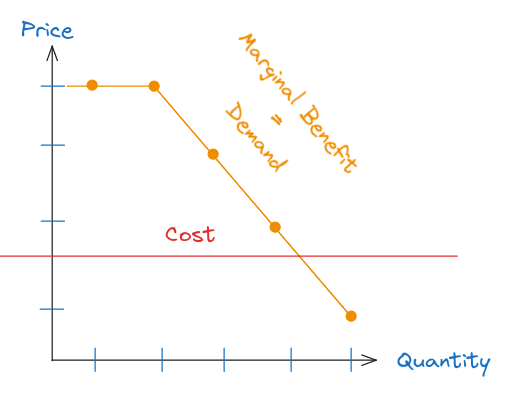
As shown in the data, the more chocolates Sam consumes, the more “satiated” he becomes (stomach might be full, enough sugar for the day, etc). Due to this, their demand for the item “diminishes” until: $$\text{Marginal Benefit}= \text{Cost}$$
Therefore, Sam should stop buying chocolate after 4 since he will be willing to pay only $0.25 for the 5th chocolate which is worth $0.40.
Ceteris Paribus
This means “Holding other things constant” in Latin
There are many extraneous factors that may affect someone’s demand curve. If Sam lost his job, he may not want to spend as much on chocolate.
Due to this, economists try to remove all other factors and focus on price.
- After that is resolved, they introduce new factors separately
The Law of Demand
The tendency for quantity to be higher when price is lower
Pretty simple:
- as prices fall
- quantity demand increases
This is so commonly found that economists often try to find exceptions to this rule.
Your Demand Curve
Demand curves are often used in tandem with other core economic principles.
Applying core principles
Let’s look back at Sam’s example and apply the core principles to his case:
- Marginal Principle: Instead of “How many chocolates?”, think “Can I get one more chocolate?”
- Cost-Benefit Principle: If Benefits higher than Cost in a Marginal Choice, buy chocolate!
- Opportunity Cost Principle: What else could Sam buy other than chocolate?
- Maybe Ice Cream? If not, how much value am I giving up for chocolate?
Rational Rule for Buyer
Buy more if marginal benefit of an item is greater or equal to price.
- Keep doing so until $$\text{Price}=\text{Marginal Benefit}$$
Demand = Marginal Benefit
- Price = Marginal Benefit
- Demand is the price you’re willing to pay at a quantity
- The Price you want to pay is informed by the Marginal Benefit you recieve
Therefore Demand and Marginal Benefit curves are the same
Market Demand
Market Demand curves plot total quantity of item demanded by the market at each price
- This gives businesses an idea of demand and pricing
Four Steps to Estimate Market Demand
- Survey: Ask everyone quantity they buy at each price
- Sum: For each price point, add up total quantites from all customers
- Scale: Raise quantities to represent entire market
- Plot: Make a curve of total quantity at each price
Market Demand Curve
These curves are downward sloping based on the Law of Demand
- Low prices attract current customers more + bring new customers into market
If there is a change in price, simply move along the curve to the desired quanity
- You DO NOT need to create a new curve and survey to see price impact
- As price changes and a point on the demand curve moves, change in quantity is demanded
Personal Note
- I left out the last part of today’s lecture (Beginning of Demand Curve Shifts) because it’s more cohesive to sum it up with the next lecture.
- This lecture was pretty fun, the prof abused a poor guy with a bunch of chocolate